Accuracy is not everything

Ever since we’ve had a patent search, we've been seeking ways to increase the accuracy. The tweaks to deep learning models and knowledge graph parsing have been the main sources for the improvements. In April 2019 we had just built a system that collects difficult graphs, the training samples that the neural net has hard time classifying correctly. With the help of this system, we had found many graph parsing fixes. Now though, the samples had started to look hard for us too. What next? We needed better tools for understanding the bottlenecks of our algorithms.

Together with the need for understanding came another thought. From the user’s point of view, finding the first good result is what matters. More accurate search means more value, but similarly, what if you could see only one or two paragraphs of relevant content per result, instead of the 30 page patent text? You could go through more results with the same effort, in practice increasing the search usefulness. If we can understand why the machine chooses a certain result, it's also easier to trust the machine. It was time to make the search explainable!

Building the explainability

Explainable AI (XAI) is a hot topic, but more so for images, and there is not much research for textual data. With just natural language, the problem is difficult. You can look at all the words separately. Then long texts will be very hard, and another question is, how enlightening can it ever be for the user to only get some words highlighted. You could also try to generate text for the explanation. Could work I guess, but that is not an easy task. Our graph model serves us well here, as we can focus on the nodes, which we only have a reasonable number.

Shapley value approximation was the natural starting point. We calculate how much the score changes if we remove a node from tree. And the calculation is simple: we try out replacing every node with random noise, and the changes in the score are our Shapley approximations. This worked. Our AI developer Sebastian created the code in couple of days, and we had something fascinating at our hands. The only problem was the speed. Processing through a 1000 node graph took 30 seconds, which would be unusable and make the production environment complex and expensive. We had ideas for optimisations but nothing ground breaking. One of the long term ideas is to make the result list explainable as well, so that you could see right away a quick summary why any of the result matters. That would mean processing not one but 50-100 graphs at a time.

Going back to the basics

I like to walk to the office. Usually I either fine-tune my mood with music, or listen e-books or podcasts, but that day there were no distractions. Could we calculate all the node scores on a single run? Finding an answer to that question is not that hard, but some ambition was needed to even thinking about it.

When we train a deep learning model, we first calculate the forward step that gives the predicted score. Then we calculate the loss, i.e. how much the score is off from the target. After that comes the backward step: the loss is carried back to affect the weights of the model. And here you may already see the simple idea. How much loss comes back to a node tells us how important that node is!

“Sebastian, I’ve got something that might be completely mad”. Not the first or last time to start a day like that. The idea was just a hunch. And it seemed to be too simple and effective to exist. Conceptually simple, that is, as if we needed to reimplement the whole backward step, this wouldn’t be easy. Luckily we avoided that, as Sebastian came up with a brilliant solution that was only possible because of PyTorch. Couple of years ago with the inferior tools, implementing the algorithm could have meant months instead of weeks. Sebastian also found out that these gradient based method are known as the saliency score in the literature. Most material comes from the work with images, one good overview is this Qure.ai blog post. The results of this saliency score based approach were about as good as with the Shapley value approximation, and fast.

You can try it!

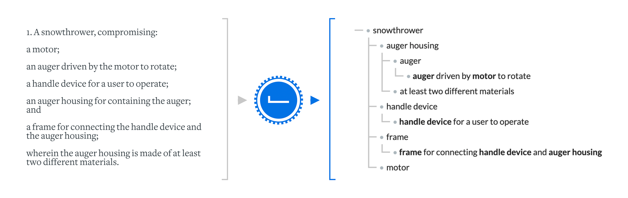
We implemented the explainable patent search as a slider that can simplify the result graph. Last remaining pieces are the nodes that the neural net considers the most relevant, in addition to the dependent nodes (parent nodes and nodes referenced from the relevant nodes). Below you can try it! The complete graph is what we parse automatically from US20170152638A1 and when you move the slider, anything unrelated to the first claim (also seen in the pictures above) will fade away. The sample application should work with any desktop browser.